This forum is disabled, please visit https://forum.opencv.org
| | 1 | initial version |
I have written in this answer some experimentations I did to understand more the concept of homography. Even if this is not really an answer of the original post, I hope it could also be useful to other people and it is a good way for me to summarize all the information I gathered. I have also added the necessary code to check and make the link between the theory and the practice.
What is the homography matrix?
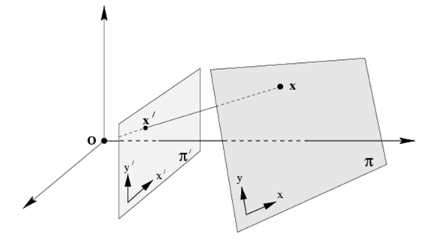
For the theory, just refer to a computer vision course (e.g. Lecture 16: Planar Homographies, ...) or book (e.g. Multiple View Geometry in Computer Vision, Computer Vision: Algorithms and Applications, ...). Quickly, the planar homography relates the transformation between two planes (up to a scale):
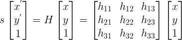
This planar transformation can be between:
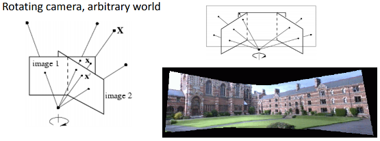
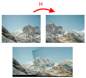
How the homography can be useful?
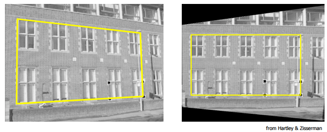
Demo 1: perspective correction
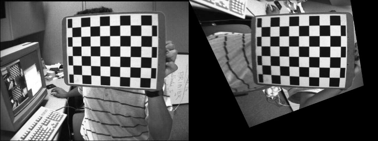
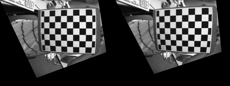
The function findChessboardCorners() returns the chessboard corners location (the left image is the source, the right image is the desired perspective view):
The homography matrix can be estimated with findHomography() or getPerspectiveTransform():
H:
[0.3290339333220102, -1.244138808862929, 536.4769088231476;
 0.6969763913334048, -0.08935909072571532, -80.34068504082408;
 0.00040511729592961, -0.001079740100565012, 0.9999999999999999]
The first image can be warped to the desired perspective view using warpPerspective() (left: desired perspective view, right: left image warped):
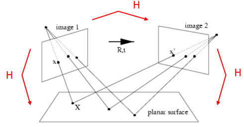
Demo 2: compute the homography matrix from the camera displacement
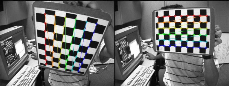
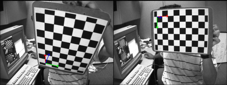
With the function solvePnP(), we can estimate the camera poses (rvec1, tvec1 and rvec2, tvec2) for the two images and draw the corresponding object frames:
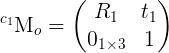
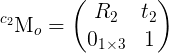

It is then possible to use the camera poses information to compute the homography transformation related to a specific object plane:
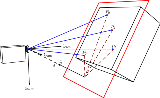
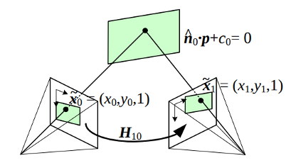
By Homography-transl.svg: Per Rosengren derivative work: Appoose (Homography-transl.svg) CC BY 3.0, via Wikimedia Commons
On this figure, n is the normal vector of the plane and d the distance between the camera frame and the plane along the plane normal. The equation to compute the homography from the camera displacement is:
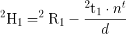
Where  is the homography matrix that maps the points in the first camera frame to the corresponding points in the second camera frame,
 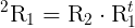 is the rotation matrix that represents the rotation between the two camera frames and
 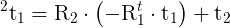 the translation vector between the two camera frames.
Here the normal vector n is the plane normal expressed in the camera frame 1 and can be computed as the cross product of 2 vectors (using 3 non collinear points that lie on the plane) or in our case directly with:
  cv::Mat normal = (cv::Mat_<double>(3,1) << 0, 0, 1);
  cv::Mat normal1 = R1*normal;
The distance d can be computed as the dot product between the plane normal and a point on the plane or by computing the plane equation and using the D coefficient:
  cv::Mat origin(3,1,CV_64F,cv::Scalar(0));
  cv::Mat origin1 = R1*origin + tvec1;
  double d_inv1 = 1.0 / normal1.dot(-origin1);
The final homography matrix that can be used to warp the first image into the desired perspective view is (the same camera is used in both images here): 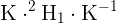
cv::Mat homography = cameraMatrix * (R_1to2-d_inv1*tvec_1to2*normal1.t()) * cameraMatrix.inv();
homography /= homography.at<double>(2,2);
The result is:
homography:
[0.416056997554822, -1.306889022302135, 553.7055454434186;
 0.7917584236503302, -0.06341244862332501, -108.2770023399513;
 0.000592635728708199, -0.00102065172420853, 0.9999999999999999]
With the same visual result (left: warp from findHomography(), right: warp from the homography computed from the camera displacement:
Demo 3: decompose the homography matrix to a camera displacement
OpenCV 3 contains the function decomposeHomographyMat() which allows to decompose the homography matrix to a set or rotations, translations and plane normals:
  std::vector<cv::Mat> Rs_decomp, ts_decomp, normals_decomp;
  cv::decomposeHomographyMat(homography, cameraMatrix, Rs_decomp, ts_decomp, normals_decomp);
The "correct" results are:
rvec_1to2=[-0.09198300622505946, -0.5372581099787472, 1.310868859706331]
t_1to2=[0.1578091503401751, 0.005603438955404258, 0.1383378923943395]
normal1: [0.1973513036075573, -0.6283452083012302, 0.7524857222361636]
The four solutions are:
Rs_decomp[0]=[-0.09198300622506073, -0.5372581099787442, 1.310868859706334]
ts_decomp[0]=[-0.7747960949402362, -0.0275112223310486, -0.6791979969371286]
normals_decomp[0]=[-0.1973513036075609, 0.6283452083012311, -0.7524857222361622]

Rs_decomp[1]=[-0.09198300622506073, -0.5372581099787442, 1.310868859706334]
ts_decomp[1]=[0.7747960949402362, 0.0275112223310486, 0.6791979969371286]
normals_decomp[1]=[0.1973513036075609, -0.6283452083012311, 0.7524857222361622]

Rs_decomp[2]=[0.1053487857879288, -0.1561929289949728, 1.401356547596018]
ts_decomp[2]=[-0.4666552464032777, 0.1050033058302994, -0.9130076461351245]
normals_decomp[2]=[-0.3131715295480532, 0.842120625125061, -0.4390403692367126]

Rs_decomp[3]=[0.1053487857879288, -0.1561929289949728, 1.401356547596018]
ts_decomp[3]=[0.4666552464032777, -0.1050033058302994, 0.9130076461351245]
normals_decomp[3]=[0.3131715295480532, -0.842120625125061, 0.4390403692367126]
According to the documentation:
At least two of the solutions may further be invalidated if point correspondences are available by applying positive depth constraint (all points must be in front of the camera).
The translation is recovered up to a scale factor (same conclusion in this post) that corresponds in fact to the distance d. All the four solutions provide here a visually correct warping:
cv::Mat homography_decomp_original = computeHomography(Rs_decomp[i], ts_decomp[i], -1.0, normals_decomp[i]); //formula to compute H from the camera displacement
cv::Mat homography_decomp = cameraMatrix * homography_decomp_original * cameraMatrix.inv();
homography_decomp /= homography_decomp.at<double>(2,2);
The homography matrix reconstructed for the first solution is:
homography_decomp:
[0.4160569975548221, -1.306889022302135, 553.7055454434186;
 0.7917584236503303, -0.06341244862332487, -108.2770023399513;
 0.0005926357287081991, -0.00102065172420853, 1]
| | 2 | No.2 Revision |
I have written in this answer some experimentations I did to understand more the concept of homography. Even if this is not really an answer of the original post, I hope it could also be useful to other people and it is a good way for me to summarize all the information I gathered. I have also added the necessary code to check and make the link between the theory and the practice.
What is the homography matrix?
For the theory, just refer to a computer vision course (e.g. Lecture 16: Planar Homographies, ...) or book (e.g. Multiple View Geometry in Computer Vision, Computer Vision: Algorithms and Applications, ...). Quickly, the planar homography relates the transformation between two planes (up to a scale):
This planar transformation can be between:
How the homography can be useful?
Demo 1: perspective correction
The function findChessboardCorners() returns the chessboard corners location (the left image is the source, the right image is the desired perspective view):
The homography matrix can be estimated with findHomography() or getPerspectiveTransform():
H:
[0.3290339333220102, -1.244138808862929, 536.4769088231476;
 0.6969763913334048, -0.08935909072571532, -80.34068504082408;
 0.00040511729592961, -0.001079740100565012, 0.9999999999999999]
The first image can be warped to the desired perspective view using warpPerspective() (left: desired perspective view, right: left image warped):
Demo 2: compute the homography matrix from the camera displacement
With the function solvePnP(), we can estimate the camera poses (rvec1, tvec1 and rvec2, tvec2) for the two images and draw the corresponding object frames:
It is then possible to use the camera poses information to compute the homography transformation related to a specific object plane:
By Homography-transl.svg: Per Rosengren derivative work: Appoose (Homography-transl.svg) CC BY 3.0, via Wikimedia Commons
On this figure, n is the normal vector of the plane and d the distance between the camera frame and the plane along the plane normal. The equation equation to compute the homography from the camera displacement is:
Where is the homography matrix that maps the points in the first camera frame to the corresponding points in the second camera frame, is the rotation matrix that represents the rotation between the two camera frames and the translation vector between the two camera frames.
Here the normal vector n is the plane normal expressed in the camera frame 1 and can be computed as the cross product of 2 vectors (using 3 non collinear points that lie on the plane) or in our case directly with:
  cv::Mat normal = (cv::Mat_<double>(3,1) << 0, 0, 1);
  cv::Mat normal1 = R1*normal;
The distance d can be computed as the dot product between the plane normal and a point on the plane or by computing the plane equation and using the D coefficient:
  cv::Mat origin(3,1,CV_64F,cv::Scalar(0));
  cv::Mat origin1 = R1*origin + tvec1;
  double d_inv1 = 1.0 / normal1.dot(-origin1);
The final homography matrix that can be used to warp the first image into the desired perspective view is (the same camera is used in both images here):
cv::Mat homography = cameraMatrix * (R_1to2-d_inv1*tvec_1to2*normal1.t()) * cameraMatrix.inv();
homography /= homography.at<double>(2,2);
The result is:
homography:
[0.416056997554822, -1.306889022302135, 553.7055454434186;
 0.7917584236503302, -0.06341244862332501, -108.2770023399513;
 0.000592635728708199, -0.00102065172420853, 0.9999999999999999]
With the same visual result (left: warp from findHomography(), right: warp from the homography computed from the camera displacement:
Demo 3: decompose the homography matrix to a camera displacement
OpenCV 3 contains the function decomposeHomographyMat() which allows to decompose the homography matrix to a set or rotations, translations and plane normals:
  std::vector<cv::Mat> Rs_decomp, ts_decomp, normals_decomp;
  cv::decomposeHomographyMat(homography, cameraMatrix, Rs_decomp, ts_decomp, normals_decomp);
The "correct" results are:
rvec_1to2=[-0.09198300622505946, -0.5372581099787472, 1.310868859706331]
t_1to2=[0.1578091503401751, 0.005603438955404258, 0.1383378923943395]
normal1: [0.1973513036075573, -0.6283452083012302, 0.7524857222361636]
The four solutions are:
Rs_decomp[0]=[-0.09198300622506073, -0.5372581099787442, 1.310868859706334]
ts_decomp[0]=[-0.7747960949402362, -0.0275112223310486, -0.6791979969371286]
normals_decomp[0]=[-0.1973513036075609, 0.6283452083012311, -0.7524857222361622]

Rs_decomp[1]=[-0.09198300622506073, -0.5372581099787442, 1.310868859706334]
ts_decomp[1]=[0.7747960949402362, 0.0275112223310486, 0.6791979969371286]
normals_decomp[1]=[0.1973513036075609, -0.6283452083012311, 0.7524857222361622]

Rs_decomp[2]=[0.1053487857879288, -0.1561929289949728, 1.401356547596018]
ts_decomp[2]=[-0.4666552464032777, 0.1050033058302994, -0.9130076461351245]
normals_decomp[2]=[-0.3131715295480532, 0.842120625125061, -0.4390403692367126]

Rs_decomp[3]=[0.1053487857879288, -0.1561929289949728, 1.401356547596018]
ts_decomp[3]=[0.4666552464032777, -0.1050033058302994, 0.9130076461351245]
normals_decomp[3]=[0.3131715295480532, -0.842120625125061, 0.4390403692367126]
According to the documentation:
At least two of the solutions may further be invalidated if point correspondences are available by applying positive depth constraint (all points must be in front of the camera).
The translation is recovered up to a scale factor (same conclusion in this post) that corresponds in fact to the distance d. All the four solutions provide here a visually correct warping:
cv::Mat homography_decomp_original = computeHomography(Rs_decomp[i], ts_decomp[i], -1.0, normals_decomp[i]); //formula to compute H from the camera displacement
cv::Mat homography_decomp = cameraMatrix * homography_decomp_original * cameraMatrix.inv();
homography_decomp /= homography_decomp.at<double>(2,2);
The homography matrix reconstructed for the first solution is:
homography_decomp:
[0.4160569975548221, -1.306889022302135, 553.7055454434186;
 0.7917584236503303, -0.06341244862332487, -108.2770023399513;
 0.0005926357287081991, -0.00102065172420853, 1]
Note: there is a minor difference between the Wikipedia source and the reference paper of decomposeHomographyMat() (Deeper understanding of the homography decomposition for vision-based control):
H = R - tn/d on Wikipedia but H = R + tn/d in the paperIt looks like it is just a difference between my understanding or the convention used (maybe in the computation/sign of d?), to be checked.